Tracks
Track groups based on file types and localtions of the track files
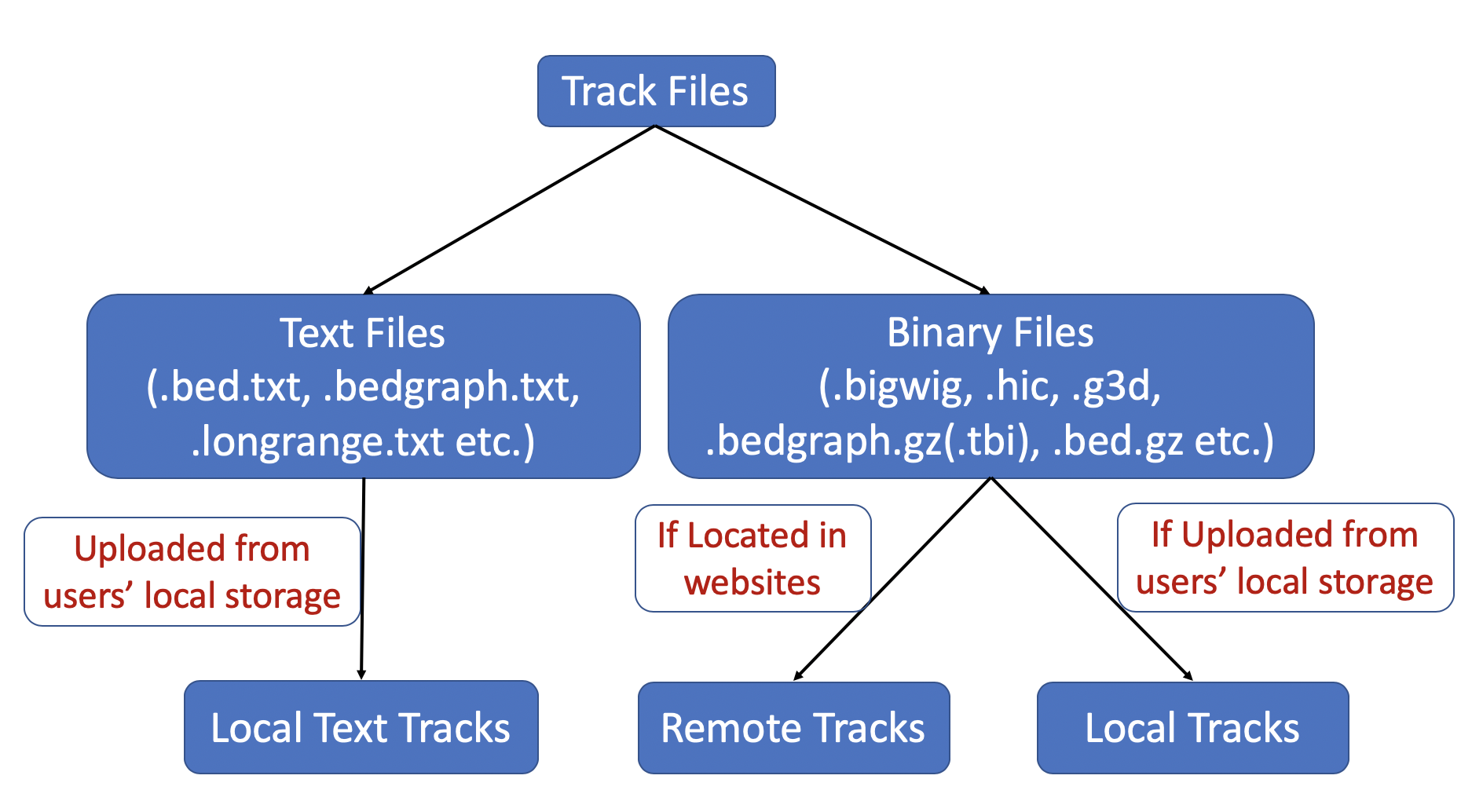
Track files are divided to 2 groups based on their file types, text format files and binary files like bigWig and hic.
For binary track files, if the track files are located at websites, they are Remote Tracks, if they are located in users’ computer then
they are Local Tracks. For text track files, right now they can be uploaded from users’ computer, they are called Local Text Tracks. Please check the following diagram as well:
Important
Since all remote tracks are hosted on the web with HTTP/HTTPS links provided for submission as tracks, the webservers which are hosting the track files need Cross-Origin Resource Sharing (CORS) enabled.
Quoted from MDN:
Cross-Origin Resource Sharing (CORS) is a mechanism that uses additional
HTTP headers to tell a browser to let a web application running at
one origin (domain) have permission to access selected resources
from a server at a different origin. A web application makes
cross-origin HTTP request when it requests a resource that has
a different origin (domain, protocol, and port) than its own origin.
Configure your webserver to enable CORS
Most likely the browser domain is different from the server the tracks are hosted on. The hosting server needs CORS enabled. For any Apache web server, you might try the either following approach.
Enable CORS on Apache2 under Ubuntu
For an Apache web server in Ubuntu this setup (add this to the enabled .conf file) would work:
Header always set Access-Control-Allow-Origin "*"
Header always set Access-Control-Allow-Headers: Range
Header always set Access-Control-Max-Age: 86400
Then restart your Apache server.
Enable CORS on Apache2 under CentOS
Try add this to the main configuration file /etc/httpd/conf/httpd.conf:
Header always set Access-Control-Allow-Origin "*"
Header always set Access-Control-Allow-Headers: Range
Header always set Access-Control-Max-Age: 86400
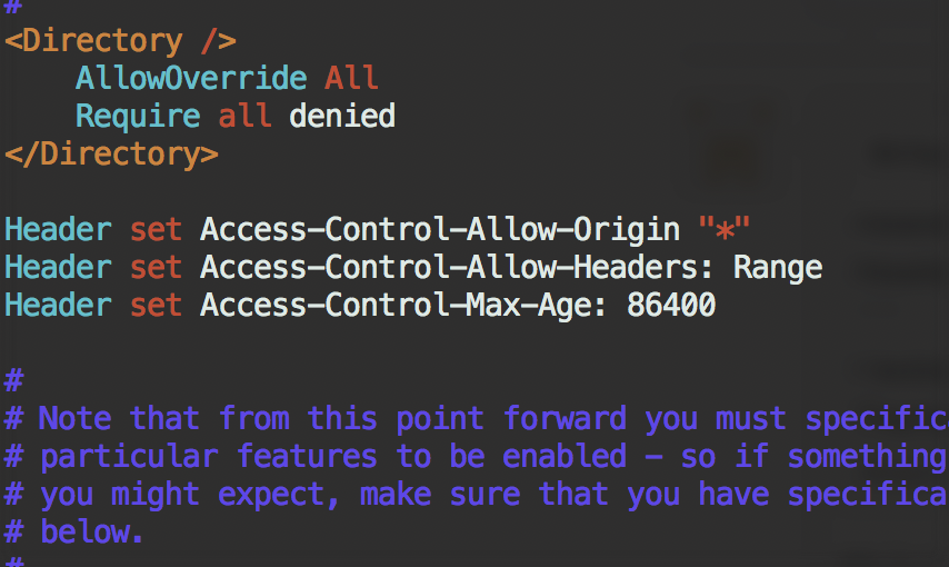
in /etc/httpd/conf.modules.d/00-base.conf, the header module should be enabled:

Then restart your Apache server.
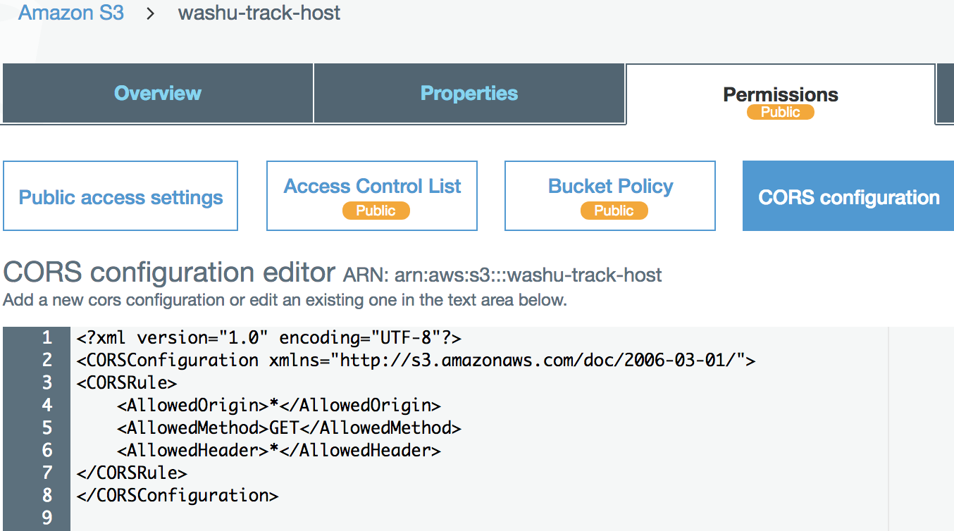
Enable CORS on Amazon S3 bucket
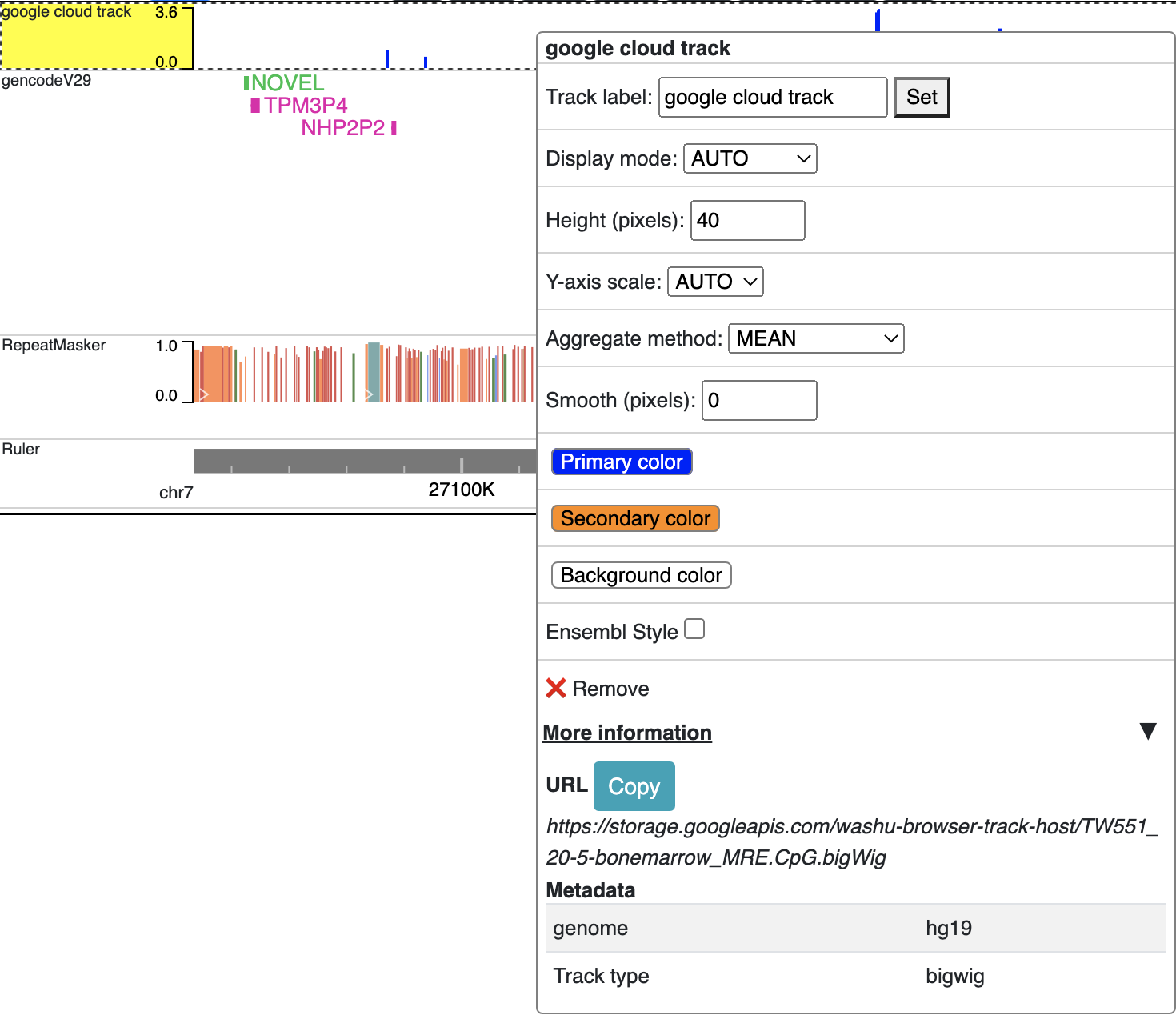
We have setup a test s3 bucket at http://washu-track-host.s3-website-us-east-1.amazonaws.com and tried bigWig files, the link http://washu-track-host.s3-website-us-east-1.amazonaws.com/bigwig/TW551_20-5-bonemarrow_MRE.CpG.bigWig can be displayed at the browser with following CORS setup:
[
    {
        "AllowedHeaders": [
            "*"
        ],
        "AllowedMethods": [
            "GET",
            "HEAD"
        ],
        "AllowedOrigins": [
            "*"
        ]
    }
]
If you happen to use old XML settings, you can setup it like this:
<?xml version="1.0" encoding="UTF-8"?>
<CORSConfiguration xmlns="http://s3.amazonaws.com/doc/2006-03-01/">
<CORSRule>
    <AllowedOrigin>*</AllowedOrigin>
    <AllowedMethod>GET</AllowedMethod>
    <AllowedHeader>*</AllowedHeader>
</CORSRule>
</CORSConfiguration>
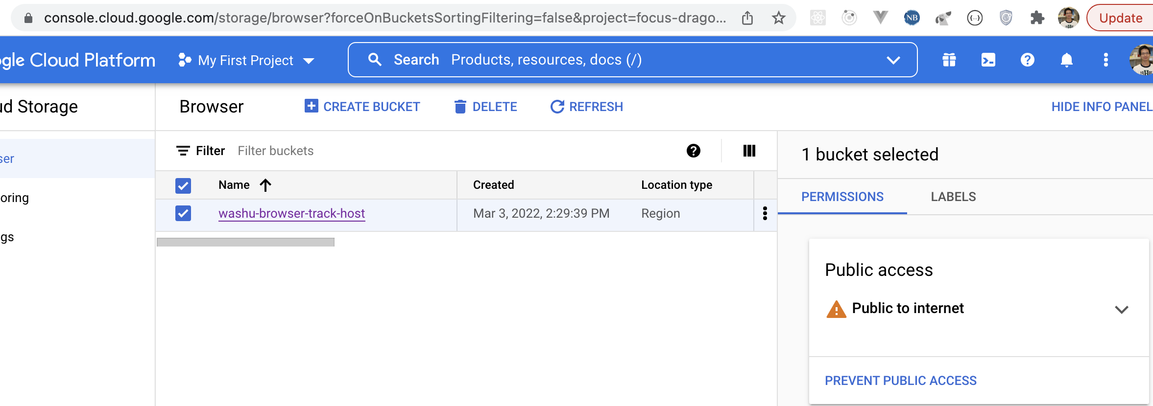
Enable CORS on Google cloud storage
If you have track files hotsed in Google cloud storage, they can be viewed in the browser as well after setting up correct CORS policy.
First you need make the bucket public, for more information you can check the docs from google:
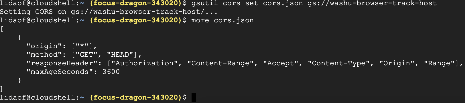
Then you can use either the gsutil tool or the CloudShell in your Google cloud’s web console. Create a file called cors.json with contents below:
[
    {
    "origin": ["*"],
    "method": ["GET", "HEAD"],
    "responseHeader": ["Authorization", "Content-Range", "Accept", "Content-Type", "Origin", "Range"],
    "maxAgeSeconds": 3600
    }
]
then set the CORS policy to your bucket with the command below:
gsutil cors set cors.json gs://washu-browser-track-host
the screenshot below shows how I did in CloudShell in the console web page:
After this, you can copy the URL to the file and submit to the browser for visualization.
Prepare track files
The browser accesses track files from their URL. Only a portion of the data, that within the specific view region, are transferred to the browser for visualization. Thus, all the track files need be hosted in a web accssible location using HTTP or HTTPS. The following sections introduce the track types that the browser supports.
Binary track file formats like bigWig and HiC can be used directly with the browser.
bedGraph, methylC, categorical, longrange and bed track files need to
be compressed by bgzip and indexed by tabix for use by the browser.
The resulting index file with suffix .tbi needs to be located
at the same URL with the .gz file.
Bed like format track files need be sorted before submission. For example, if we have a track file named track.bedgraph
we can use the generic Linux sort command, the bedSort tool from UCSC, or the sort-bed command from BEDOPS.
Here is an example command using each of the three methods:
# Using Linux sort
sort -k1,1 -k2,2n track.bedgraph > track.bedgraph.sorted
# Using bedSort
bedSort track.bedgraph track.bedgraph.sorted
# Using sort-bed
sort-bed track.bedgraph > track.bedgraph.sorted
Then the file must be compressed using bgzip and indexed using tabix:
bgzip track.bedgraph.sorted
tabix -p bed track.bedgraph.sorted.gz
Move files “track.bedgraph.sorted.gz” and “track.bedgraph.sorted.gz.tbi” to a web server. The two files must be in the same directory. Obtain the URL to “track.bedgraph.sorted.gz” for submission.
SAM files first need to be compressed to BAM files. BAM files need to be coordinate sorted and
indexed for use by the browser.
The resulting index file with suffix .bai needs be located
at the same URL with the .bam file.
Here is an example command:
# Using samtools view to convert to bam
samtools view -Sb test.sam > test.bam
# Using samtools sort to coordinate sort the file
samtools sort test.bam > test.sorted.bam
# Using samtools index
samtools index test.sorted.bam
Annotation Tracks
Annotation tracks represent genomic features or intervals across the genome. Popular examples include SNP files, CpG Island files, and blacklisted regions.
bed
bed format files can be used to annotate elements across the genome or to represent reads from a sequencing experiment.
For more about the bed format please check the UCSC bed page.
Example lines are below:
chr9        3035610 3036180 Blacklist_155   .       +
chr9        3036200 3036480 Blacklist_156   .       +
chr9        3036420 3036660 Blacklist_157   .       +
Every line must consist of at least 3 fields separated by the Tab delimiter. The required fields from
left to right are chromosome, start position (0-based), and end position (not included).
A fourth (optional) column is reserved for the name of the interval and the sixth column (optional)
is reserved for the strand. All other columns are ignored, but can be present in the file.
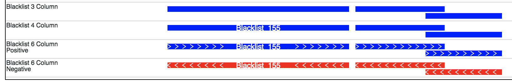
Note
The display of a bed file differs by how many columns are provided in the file
(see image above). The simplest, 3 column, format just displays blocks for
each interval. The four column format displays the name of each element over each interval.
If the sixth column is provided in the file then >>> or <<< will be displayed over
each interval to represent strand information.
This format needs to be compressed by bgzip and indexed by tabix for submission as a track. See Prepare track files.
bigbed
bigbed is a binary format of bed file. bigbed file can be submitted directly without bgzip/tabix processing. For more about the bed format please check the UCSC bigbed page.
refbed
The refbed format files allows you to upload a custom gene annotation track. It is similar to the
refGene bed-like file downloaded from UCSC but with slight modifications. Each file of
this format contains (each column is separated by Tab):
chr, transcript_start, transcript_stop, translation_start, translation_stop, strand, gene_name, transcript_id, type, exon(including UTR bases) starts, exon(including UTR bases) stops, and additional gene info (optional)
This format needs to be compressed by bgzip and indexed by tabix for submission as a track. See Prepare track files.
Hint
The 9th column contains gene type, but is simplified from the Gencode/Ensembl annotations to coding, pseudo, nonCoding, problem, and other. These classes of gene type are colored differently when the track is displayed on the browser.
Hint
The 10th and 11th columns contain exon starts and ends respectively. Each start or end is seperated by a comma.
For example:
start1,start2,start3,start4 stop1,stop2,stop3,stop4
100,120,140,160 110,130,150,170
Hint
The 12th column contains extra information. This information can be manually annotated or we suggest using Ensembl Biomart to download paired Transcript stable IDs and Gene descriptions. The information in this column must be seperated by spaces and not tabs.
All of the below lines will work for additional information in the 12th column:
Gene ID:ENSMUSG00000103482.1 Gene Type:TEC Transcript Type:TEC Additional Info:predicted gene, 37999 [Source:MGI Symbol;Acc:MGI:5611227]
Gene ID:ENSMUSG00000103482.1 Gene Type:TEC Transcript Type:TEC
ENSMUSG00000103482.1 TEC
Additional Info:predicted gene, 37999 [Source:MGI Symbol;Acc:MGI:5611227]
My Favorite Gene
Here are a few example lines in refbed format from gencode.vM17.annotation.gtf (mouse mm10 format):
chr1        24910461        24911659        24910461        24911659        -       RP23-109H7.1    ENSMUST00000187022.1    pseudo  24911220,24910461       24911659,24910681       Gene       ID:ENSMUSG00000100808.1 Gene Type:processed_pseudogene Transcript Type:processed_pseudogene Additional Info:predicted gene 28594           [Source:MGI Symbol;Acc:MGI:5579300]
chr1        25203443        25205696        25203443        25205696        -       Adgrb3  ENSMUST00000190202.1    coding  25203443        25205696        Gene                             ID:ENSMUSG00000033569.17 Gene Type:protein_coding Transcript Type:retained_intron Additional Info:adhesion G protein-coupled receptor     B3 [Source:MGI Symbol;Acc:MGI:2441837]
chr1        25276404        25277954        25276404        25277954        -       RP23-21P2.4     ENSMUST00000193138.1    problem 25276404        25277954        Gene                         ID:ENSMUSG00000104257.1 Gene Type:TEC Transcript Type:TEC Additional Info:predicted gene, 20172 [Source:MGI Symbol;Acc:MGI:5012357]
chr1        26566833        26566938        26566833        26566938        +       Gm24064 ENSMUST00000157486.1    nonCoding       26566833        26566938        Gene                           ID:ENSMUSG00000088111.1 Gene Type:snoRNA Transcript Type:snoRNA Additional Info:predicted gene, 24064 [Source:MGI                         Symbol;Acc:MGI:5453841]
Note
The last optional column is dislayed as a gene description when a gene is clicked on the browser. Our modified format can be
easily obtained from available refGene.bed file downloads from UCSC. Gencode GTF and Ensembl GTF files can be manipulated to
this format using the Converting_Gencode_or_Ensembl_GTF_to_refBed.bash script in scripts. The script by default puts
Gene ID:, Gene Type:, and Transcript Type: in the additional information column. Run with an annotation file, with
columns Transcript_ID and Description (seperated by a tab), the script will also add “Additional Info” to the 12th column. The
script depends on bedtools, bgzip, and tabix. Lastly, within the script an awk array is used to reclassify gene type and
can easily be modified for additional gene types.
The script is run as follows:
bash Converting_Gencode_or_Ensembl_GTF_to_refBed.bash Ensembl my.gtf my_optional_annotation.txt
bash Converting_Gencode_or_Ensembl_GTF_to_refBed.bash Gencode gencode.vM17.annotation.gtf
bash Converting_Gencode_or_Ensembl_GTF_to_refBed.bash Gencode gencode.vM17.annotation.gtf biomart_2col.txt
Warning
Spaces are used as delimiters in the GTF files so change gene names with spaces before processing.
For Example:
sed -i 's/ (1 of many)/_(1_of_many)/g' Danio_rerio.GRCz10.91.chr.gtf
rgbpeak
rgbpeak track file is based on bigbed format, content of a rgbpeak file (in bed format) looks like below:
chr10 46092019 46092519 chr10_46092019 537 . 46092019 46092519 117,117,117
chr10 47253553 47254053 chr10_47253553 748 . 47253553 47254053 107,107,107
where the columns are chrom, start, end, peak_id, score, strand, thick_start, thick_end, RGB value, the RBG value will be used for the color while ploting and score will be used to determin the height of the peak.
if there is strand, arrow will be drew if zoom enough. thick_start and thick_end columns are ignored now.
The bed file like above can be convert to bigbed format using the commands below:
bedSort peaks_rgb.bed peaks_rgb.bed
bedToBigBed peaks_rgb.bed hg38.chroms.sizes peaks_rgb.bigbed
bedcolor
Simiar to bed track, bedcolor track is a 4 column bed file while the 4th column is a color string:
chr11       108280000       109080000       #ff0100
chr11       109080000       109480000       #0000ff
chr11       109720000       110160000       #018100
chr11       110200000       111400000       #0064fb
chr11       111400000       112640000       #ef8c0a
chr11       112640000       113480000       #7f007f
chr11       113520000       114520000       #520000
chr11       114520000       114880000       #39ae00
It can be uploaded as local text track, or indexed after bgzip/tabix and submitted as remote track.
Variant Tracks
VCF
VCF files can be visulaized in the browser for displaying variant call data. Currently VCF file need to be bgzip and tabix indexed for submission.
The VCF track has 3 display modes: auto, density and full. By default it’s on auto mode, this means when viewing a VCF track at a region greater than 100Kb, the track will be displayed as numerical track showing the density of the variant calls, and when view region is less than or equal to 100Kb, it will be displayed in Full mode.
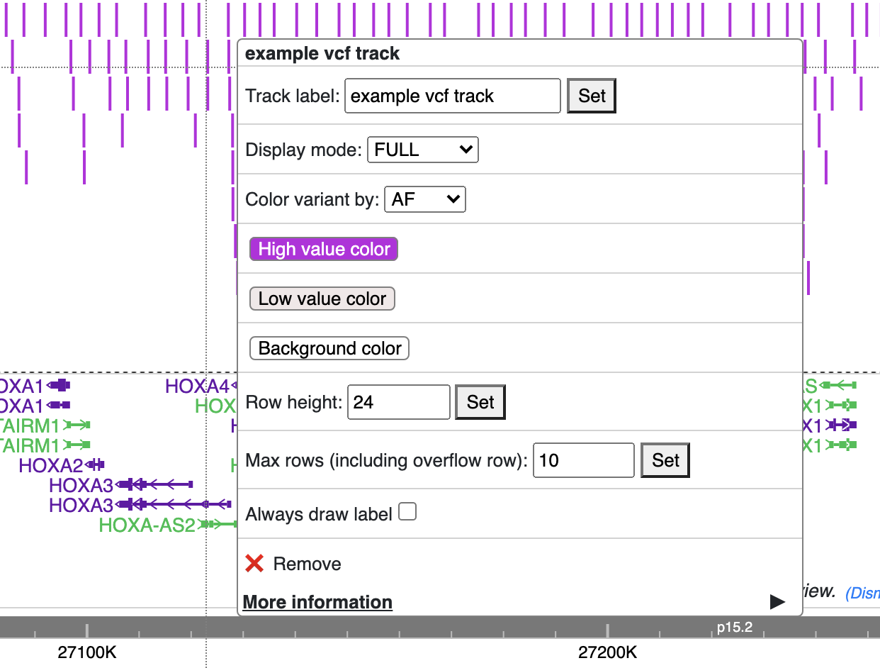
The display mode can be changed from the right clicking menu. Click each of the variant item will show the popup tooltip with more information about this variant.
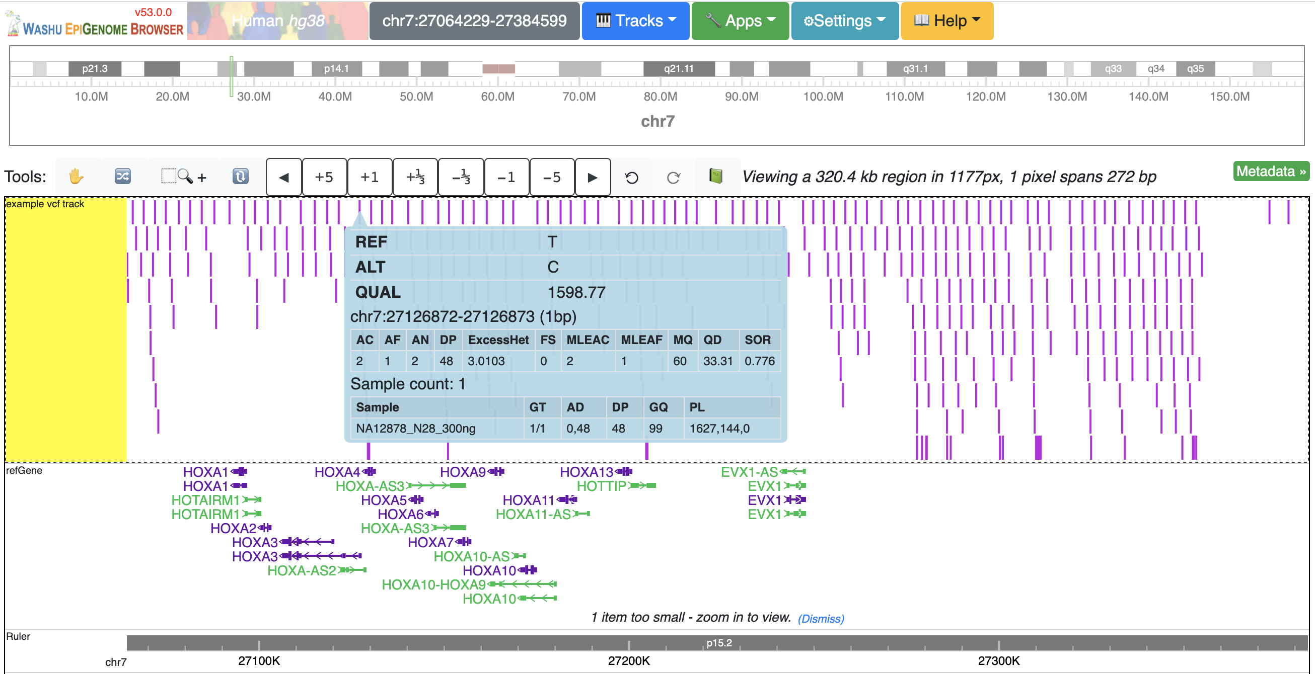
Color of each variant item are encoded based on the AF or quality value, using which value (AF or quality) to color the variant, or color of high and low value variant can be customized from right clicking menu as well.
Numerical Tracks
Currently there are two types of numerical tracks:
bigWig
bigWig is a popular format to represent numerical values over genomic coordinates.
Please check the UCSC bigWig page to learn more about this format.
bedGraph
bedGraph format also defines values in diffenent genomic locations.
For more about the bedGraph format please check the UCSC bedGraph page.
Example lines are below:
chr12   6537598 6537599 28.80914
chr12   6537599 6537600 28.96908
chr12   6537599 6537612 -2
chr12   6537600 6537601 29.30229
Every line consists of 4 fields separated by the Tab delimiter. The fields from
left to right are chromosome, start position (0-based), end position (not included), and value.
Note
You can use negative values for reverse strand. Both positive and negative
values can exist over the same coordinates (they can overlap). In bigWig format
negative values can also be specified, but they cannot overlap with positive values.
This format needs to be compressed by bgzip and indexed by tabix for submission as a track. See Prepare track files.
Dynamic Sequence Tracks
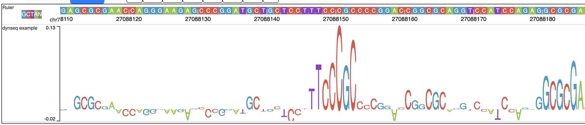
dynseq
dynseq is a new track type which is proposed and initially developped by Surag Nair from Anshul Kundaje’s lab at Stanford University.
Its track file is the same as bigWig format. It provides scores for each nucleotide in the genome, which can be derived from using importance scoring methods on machine learning models. We visualize them as a string of letters with different colors (for each nucleotide) and different heights scaled by the importance scores.
An example of loaded dynseq track highlighting an E2F motif instance is illustrated below:
Read Alignment BAM Tracks
bam
The bam format is a compressed SAM format used to store sequence alignment data.
Please check the Samtools Documentation page to learn more about this format and how to manipulate these files.
Methylation Tracks
Methylation experiments like MeDIP-seq or MRE-seq can use bigWig or bedGraph format for data display. For WGBS if users want to show read depth, methylation context, and methylation level then the data is best suited for the methylC format, described below.
methylC
Methylation data are formatted in methylC format, which is a 7 column bed format file:
chr1    10542   10543   CG      0.923   -       26
chr1    10556   10557   CHH     0.040   -       25
chr1    10562   10563   CG      0.941   +       17
chr1    10563   10564   CG      0.958   -       24
chr1    10564   10565   CHG     0.056   +       18
chr1    10566   10567   CHG     0.045   -       22
chr1    10570   10571   CG      0.870   +       23
chr1    10571   10572   CG      0.913   -       23
Each line contains 7 fields separated by Tab. The fields are
chromosome, start position (0-based), end position (not included),
methylation context (CG, CHG, CHG etc.), methylation value, strand,
and read depth.
This format needs to be compressed by bgzip and indexed by tabix for submission as a track. See Prepare track files.
Categorical Tracks
Categorical tracks represent genomic bins for different categories. The most popular example is the represnetation of chromHMM data which indicates which region is likely an enhancer, likely a promoter, etc. Other uses for the track include the display of different types of methylation (DMRs, DMVs, LMRs, UMRs, etc.) or even peaks colored by tissue type.
categorical
The categorical track uses the first three columns of the standard bed format
(chromosome, start position (0-based), and end position (not included))
with the addition of a 4th column indicating the category type which can be a string or number:
chr1    start1  end1    category1
chr2    start2  end2    category2
chr3    start3  end3    category3
chr4    start4  end4    category4
Important
when you use numbers like 1, 2 and 3 as category names, in the datahub definition,
please use it a string for the category attribute in options, see the example below:
{
    "type": "categorical",
    "name": "ChromHMM",
    "url": "https://egg.wustl.edu/d/hg19/E017_15_coreMarks_dense.gz",
    "options": {
        "category": {
            "1": {"name": "Active TSS", "color": "#ff0000"},
            "2": {"name": "Flanking Active TSS", "color": "#ff4500"},
            "3": {"name": "Transcr at gene 5' and 3'", "color": "#32cd32"}
        }
    }
}
This format needs to be compressed by bgzip and indexed by tabix for submission as a track. See Prepare track files.
Long range chromatin interaction
Long range chromatin interaction data are used to show relationships between genomic regions. HiC is used to show the results from a HiC experiment.
HiC
To learn more about the HiC format please check https://github.com/aidenlab/juicer/wiki/Data.
longrange
The longrange track is a bed format-like file type. Each row contains columns from left to right:
chromosome, start position (0-based), and end position (not included), interaction target
in this format chr2:333-444,55. As an example, interval “chr1:111-222” interacts with
interval “chr2:333-444” on a score of 55,
we will use following two lines to represent this interaction:
chr1    111 222  chr2:333-444,55
chr2    333 444  chr1:111-222,55
Important
Be sure to make TWO records for a pair of interacting loci, one record for each locus.
This format needs to be compressed by bgzip and indexed by tabix for submission as a track. See Prepare track files.
bigInteract
The bigInteract format from UCSC can also be used at the browser, for more details about this format, please check the UCSC bigInteract format page.
cool
Thanks to the higlass team who provides the data API, the browser is able to display cool tracks by using the data uuid
from the higlass server, for example, you can use the uuid Hyc3TZevQVm3FcTAZShLQg to represent the track for Aiden et al. (2009) GM06900 HINDIII 1kb,
for a full list of available cool tracks please check http://higlass.io/api/v1/tilesets/?dt=matrix
qBED Track
qBED is tab-delimited, plain text format for discrete genomic data, such as transposon insertions. This format requires a minimum of four columns and supports up to six. The four required columns are CHROM, START, END, and VALUE, where VALUE is a numeric value (i.e. an int or float). As with BED files, the START and END coordinates are 0-indexed. The fifth and sixth columns are optional and represent STRAND and ANNOTATION, respectively. The ANNOTATION column can be used to store sample- or entry- specific information, such as a replicate barcode. Here is an example of a four-column qBED file:
chr1    41954321        41954325        1
chr1    41954321        41954325        18
chr1    52655214        52655218        1
chr1    52655214        52655218        1
chr1    54690384        54690388        3
chr1    54713998        54714002        1
chr1    54713998        54714002        1
chr1    54713998        54714002        13
chr1    54747055        54747059        1
chr1    54747055        54747059        4
chr1    60748489        60748493        2
Here is an example of a six-column qBED file:
chr1    51441754        51441758        1       -       CTAGAGACTGGC
chr1    51441754        51441758        21      -       CTTTCCTCCCCA
chr1    51982564        51982568        3       +       CGCGATCGCGAC
chr1    52196476        52196480        1       +       AGAATATCTTCA
chr1    52341019        52341023        1       +       TACGAAACACTA
chr1    59951043        59951047        1       +       ACAAGACCCCAA
chr1    59951043        59951047        1       +       ACAAGAGAGACT
chr1    61106283        61106287        1       -       ATGCACTACTTC
chr1    61106283        61106287        7       -       CGTTTTTCACCT
chr1    61542006        61542010        1       -       CTGAGAGACTGG
Your text file must be sorted by the first three columns. If your filename is example.qbed, you can sort it with the following command: sort -k1V -k2n -k3n example.qbed > example_sorted.qbed
Alternatively, with bedops: sort-bed example.qbed > example_sorted.qbed
Note that you can have strand information without a barcode, but you cannot have barcode information without a strand column.
Place your sorted qBED file in a web-accessible directory, then compress and index as follows:
bgzip example_sorted.qbed
tabix -p bed example_sorted.qbed.gz
genome-align Track
genome-align is tab-delimited, plain text BED-like format to display pairwise whole-genome alignment. It can be directly derived from AXT file. The four required columns are CHROM, START, END, and ALIGNMENT, where ALIGNMENT indicates id number and detailed alignment information in a JSON format
chr1 start end alignment
The Fourth column ALIGNMENT contains the following information:
"id":1,
"genomealign": {
    "chr": "chr4",
    "start": 154100819,
    "stop": 154100880,
    "strand": "-",
    "targetseq": "ATTGGAGGAAAGATGAGTGAGAGCATCAACTTCTCTCACAACCTAGGCCAGTAAGTAGTGCTT",
    "queryseq":  "ATTGGAGGGAGGGTGAACAAAGAGATAGACTTCTG--GCAACCTGGGCCAGTAGGTAGTGTCT"
}
Here is an example of the genome-align track:
chr1    12177   12240   id:1,genomealign:{chr:"chr4",start:154100819,stop:154100880,strand:"-",targetseq:"ATTGGAGGAAAGATGAGTGAGAGCATCAACTTCTCTCACAACCTAGGCCAGTAAGTAGTGCTT",queryseq:"ATTGGAGGGAGGGTGAACAAAGAGATAGACTTCTG--GCAACCTGGGCCAGTAGGTAGTGTCT"}
chr1    12245   12273   id:2,genomealign:{chr:"chr9",start:114130992,stop:114131016,strand:"+",targetseq:"CATCTCCTTGGCTGTGATACGTGGCCGG",queryseq:"TGTCCCCTTGTCTGC----CGGGGCTGG"}
AXT file can be generated by lastz or blastz. It is also possible to make genome alignment using minimap2, and sequentially convert minimap2 SAM output to AXT file. Here is our pipeline making hg38-CHM13 genome-align AXT file:
minimap2 -x asm5 --cs=long hg38.fa chm13.fa > hg38-chm13.paf
sort -k6,6 -k8,8n -k9,9n hg38-chm13.paf|perl -ln unique_paf.pl > hg38-chm13.unique.paf
paftools.js view -f maf hg38-chm13.unique.paf > hg38-chm13.maf
maf-convert axt hg38-chm13.maf > hg38-chm13.axt
python3 axtSplit.py 100 hg38-chm13.axt hg38-chm13.split.axt
Note we used two custom script unique_paf.pl and axtSplit.py to remove redundant segments in the alignment and split long alignment records to smaller ones separated by gaps > 100bp. You can find them in the scripts directory: (https://github.com/lidaof/eg-react/blob/master/backend/scripts).
AT last, we have a script to convert AXT file to genome-align format, you can find it in the scripts directory: (https://github.com/lidaof/eg-react/blob/master/backend/scripts/axt2align.py).
Your text file must be sorted by the first three columns. If your filename is example.qbed, you can sort it with the following command: sort -k1V -k2n -k3n example.genomealign > example.sorted.genomealign
Place your sorted genome-align file in a web-accessible directory, then compress and index as follows:
bgzip example.sorted.genomealign
tabix -p bed example.sorted.genomealign.gz
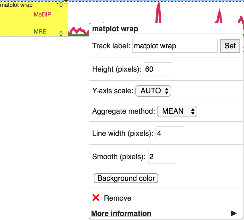
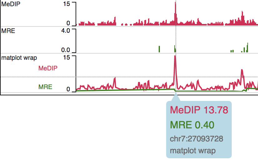
Matplot Track
A matplot (also called a line plot) displays multiple numerical tracks on the same X and Y axes to easily compare datasets. Data is plotted as curves instead of bar plots.
To use matplot, choose more than 1 numerical tracks:
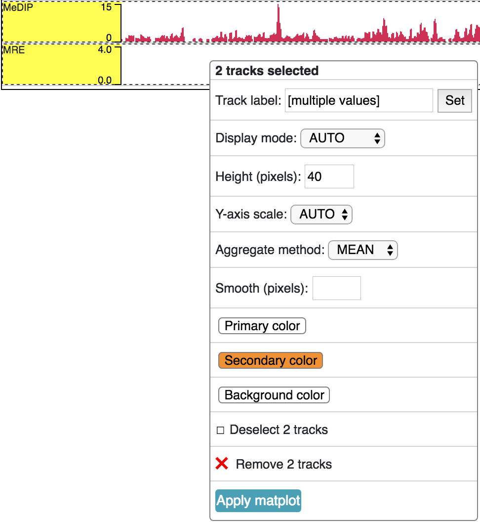
Right click, and choose Apply matplot button, The new matplot track will be shown:
and it also supports many configurations: